Código
library(tidyverse)
library(readxl)
library(infer)

theme_set(theme_bw())Inferencia sobre una población
library(tidyverse)
library(readxl)
library(infer)
theme_set(theme_bw())datos <- read_csv("../datos/Encuesta_Motociclistas.csv") |>
select(
municipio,
sexo = hombre,
nivel_educativo,
herramienta_trabajo,
experiencia,
cilin_grupo,
gasto_anual,
licencia_moto,
licencia_curso,
) |>
mutate(
municipio = str_to_title(municipio),
sexo = if_else(sexo == 1, "Hombre", "Mujer"),
herramienta_trabajo = if_else(herramienta_trabajo == 0, "No", "Sí"),
licencia_moto = if_else(licencia_moto == 0, "No", "Sí"),
licencia_curso = if_else(licencia_curso == 0, "No", "Sí"),
nivel_educativo = factor(
nivel_educativo,
c(
"Primaria o menos",
"Secundaria",
"Técnica / Tecnológica",
"Universitaria o postgrado"
)
),
experiencia = factor(experiencia, levels = c("0-2", "3-5", "6-10", "11-20", ">20")),
cilin_grupo = factor(cilin_grupo, levels = c("<100", "100-125", "126-200", ">200"))
) |>
filter(!is.na(gasto_anual))
datos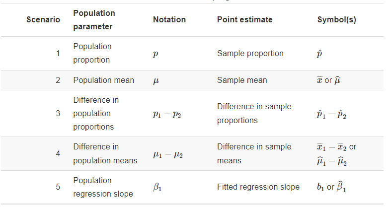


ggpubr::ggqqplot(datos$gasto_anual)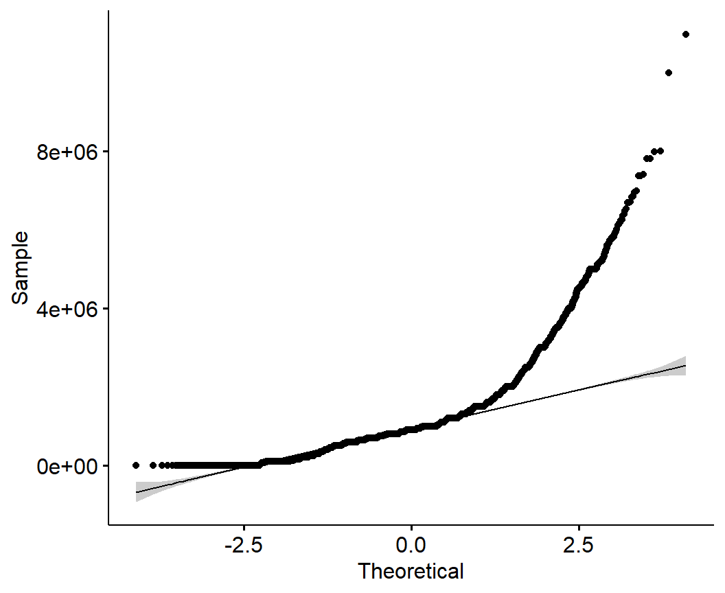
\[H_0: \mu = 1.000.000\]
\[H_1: \mu \neq 1.000.000\]
\[T = \frac{\bar{X} - \mu}{S/\sqrt{n}}\]
x_barra <- mean(datos$gasto_anual, na.rm = TRUE)
mu_referencia <- 1e+06
desviacion_muestral <- sd(datos$gasto_anual, na.rm = TRUE)
raiz_n <- sqrt(nrow(datos))
\[T = \frac{1039744 - 1000000}{713080/157.31} = 8.768062\]
(x_barra - mu_referencia) / (desviacion_muestral / raiz_n)[1] 8.768062
Podemos obtener los límites critícos con R:
qt(p = 0.025, df = nrow(datos) - 1, lower.tail = TRUE)[1] -1.96006qt(p = 0.025, df = nrow(datos) - 1, lower.tail = FALSE)[1] 1.96006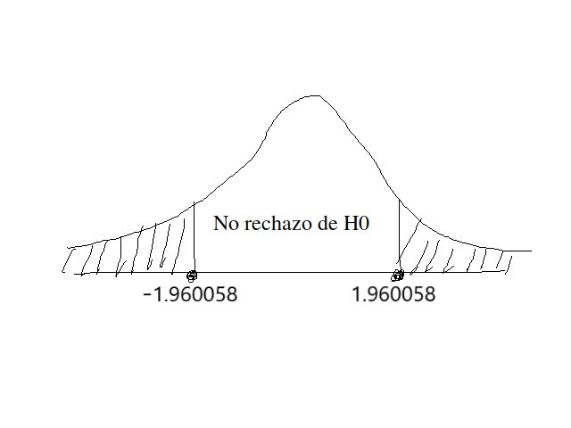
\[\bar{X} - t_{\alpha/2, n-1} \times \frac{s}{\sqrt{n}}\]
x_barra - (1.96006 * (desviacion_muestral / raiz_n))[1] 1030859\[\bar{X} + t_{\alpha/2, n-1} \times \frac{s}{\sqrt{n}}\]
x_barra + (1.96006 * (desviacion_muestral / raiz_n))[1] 1048629pt(q = -8.768062, df = nrow(datos) - 1, lower.tail = TRUE)[1] 9.661257e-19pt(q = 8.768062, df = nrow(datos) - 1, lower.tail = FALSE)[1] 9.661257e-199.661257e-19 + 9.661257e-19[1] 1.932251e-18x: la variable sobre la cual estamos haciendo inferencia. En este caso el gasto_anualalternative: tipo de hipótesis alternativa. En este es una prueba bilateral usamos “two.sided”conf.level: nivel de confianza (1 - nivel de significancia = 1 - 0.05 = 0.95)mu: valor promedio de referencia. En este caso es 1.000.000t.test(x = datos$gasto_anual,
alternative = "two.sided",
conf.level = 0.95,
mu = 1e+06)
    One Sample t-test

data:  datos$gasto_anual
t = 8.7681, df = 24747, p-value < 2.2e-16
alternative hypothesis: true mean is not equal to 1e+06
95 percent confidence interval:
 1030859 1048629
sample estimates:
mean of x
1039744 prueba_t1 <- t.test(
x = datos$gasto_anual,
alternative = "two.sided",
conf.level = 0.95,
mu = 1e+06
)
library(broom)
prueba_t1 |> tidy()wilcox.test(
x = datos$gasto_anual,
alternative = "two.sided",
conf.int = TRUE,
conf.level = 0.95,
mu = 1e+06
)
    Wilcoxon signed rank test with continuity correction

data:  datos$gasto_anual
V = 114442553, p-value < 2.2e-16
alternative hypothesis: true location is not equal to 1e+06
95 percent confidence interval:
 925000 945000
sample estimates:
(pseudo)median
935000 
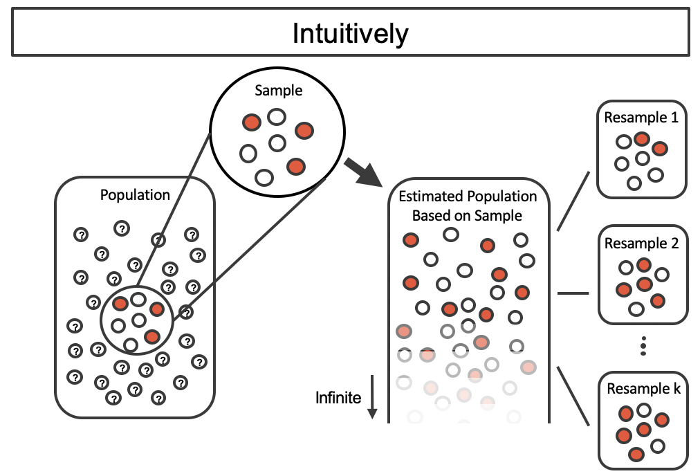
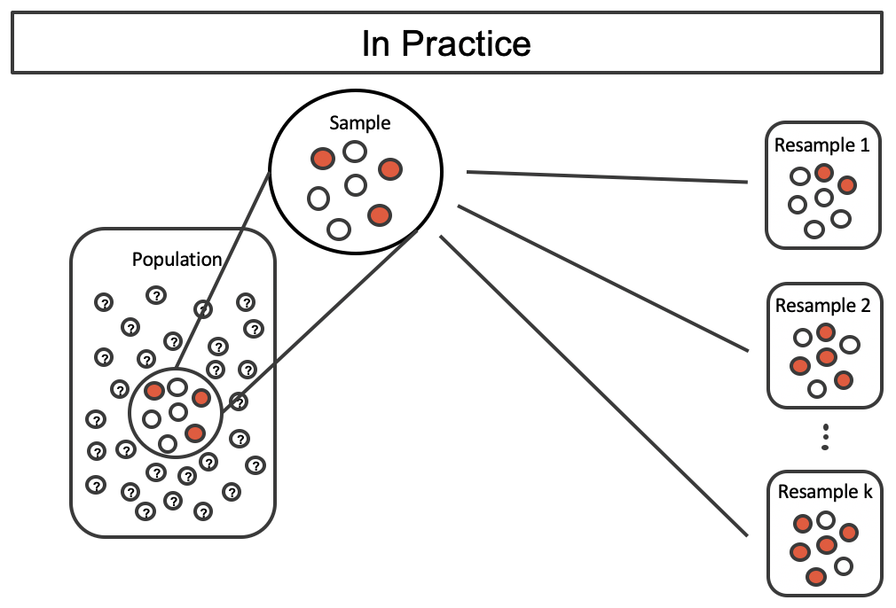
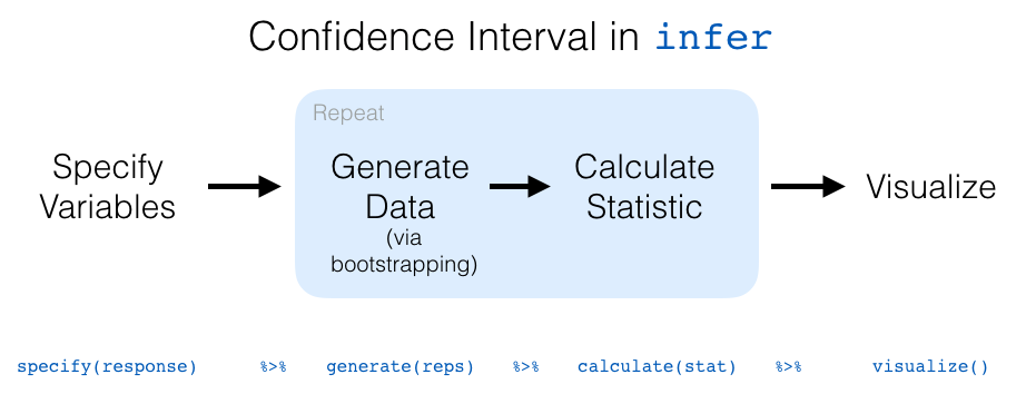
inferspecify()generate()calculate()visualize()get_confidence_interval(). Nota: para mejorar la visualización de los intervalos de confianza, se puede utilizar la función shade_confidence_interval()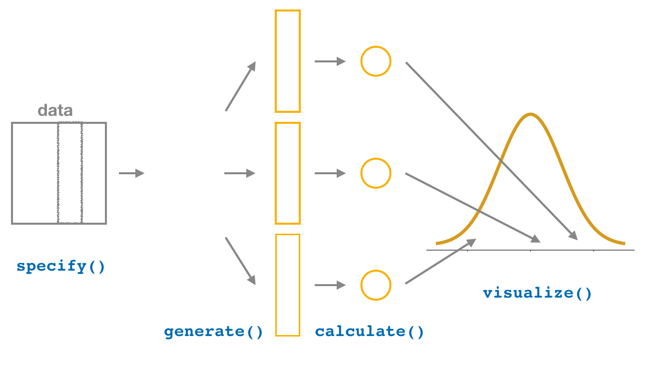
set.seed(2025)
bootstrap_gasto_anual <-
  datos |>
  specify(response = gasto_anual) |>
  generate(reps = 1000, type = "bootstrap") |>
  calculate(stat = "mean")

bootstrap_gasto_anualbootstrap_gasto_anual |>
visualize()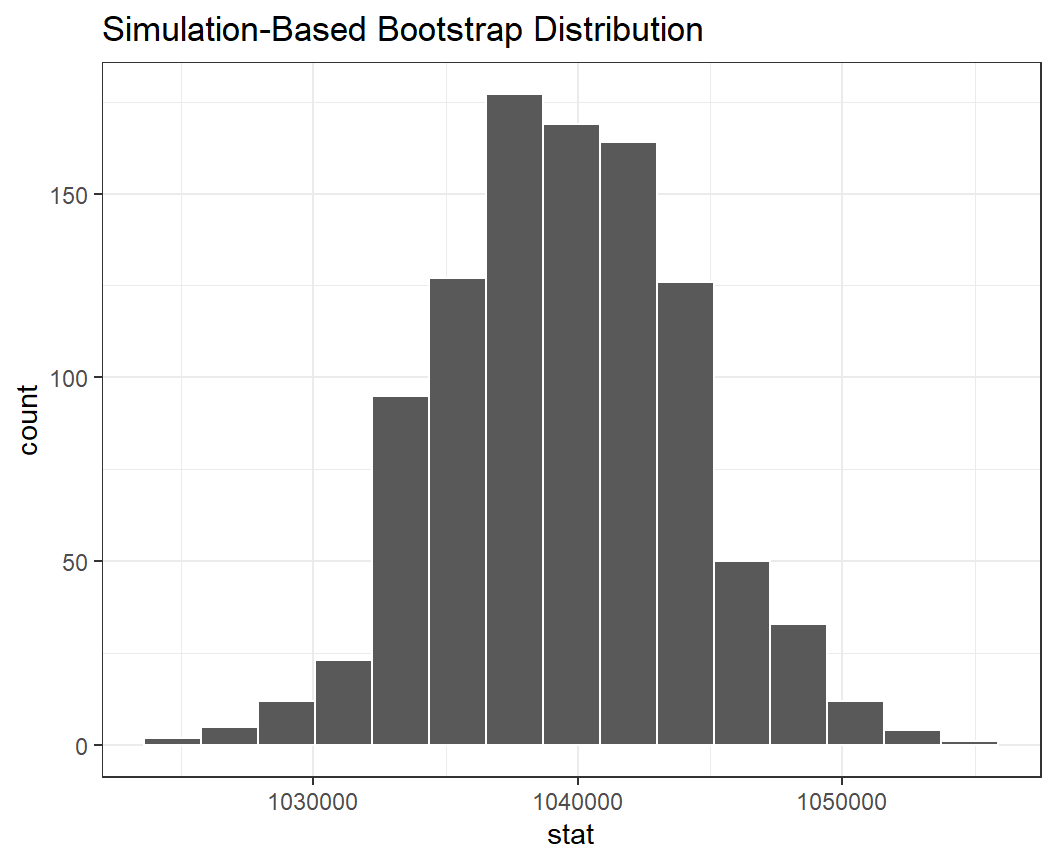
 {fig-align=“center” width = “70%”}
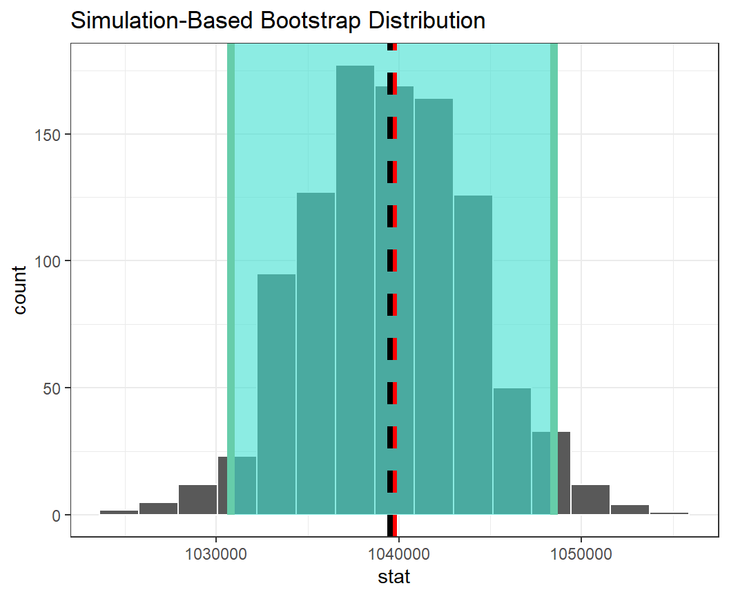
ic_promedio_percentil <-
  bootstrap_gasto_anual |>
  get_confidence_interval(level = 0.95, type = "percentile")
ic_promedio_percentilbootstrap_gasto_anual |>
visualize() +
shade_confidence_interval(endpoints = ic_promedio_percentil) +
geom_vline(
xintercept = x_barra,
color = "red",
lty = 2,
size = 1.5
) +
geom_vline(
xintercept = mean(bootstrap_gasto_anual$stat),
color = "black",
lty = 2,
size = 1.5
)
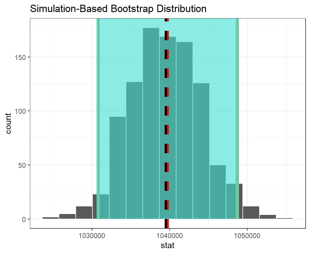
ic_promedio_error_est <-
  bootstrap_gasto_anual |>
  get_confidence_interval(type = "se", point_estimate = x_barra)
ic_promedio_error_estbootstrap_gasto_anual |>
visualize() +
shade_confidence_interval(endpoints = ic_promedio_error_est) +
geom_vline(
xintercept = x_barra,
color = "red",
lty = 2,
size = 1.5
) +
geom_vline(
xintercept = mean(bootstrap_gasto_anual$stat),
color = "black",
lty = 2,
size = 1.5
)
:::
\[H_0: p = 50\%\]
\[H_1: p \neq 50\%\]
datos2 <-
  datos |>
  filter(!is.na(licencia_curso))

datos2$licencia_curso |>
  table() |>
  prop.table()
       No        Sí
0.2835426 0.7164574 set.seed(2025)
remuestreo_licencia_curso <- datos2 |>
specify(response = licencia_curso, success = "Sí") |>
generate(reps = 1000, type = "bootstrap") |>
calculate(stat = "prop")
remuestreo_licencia_cursoremuestreo_licencia_curso |>
visualize()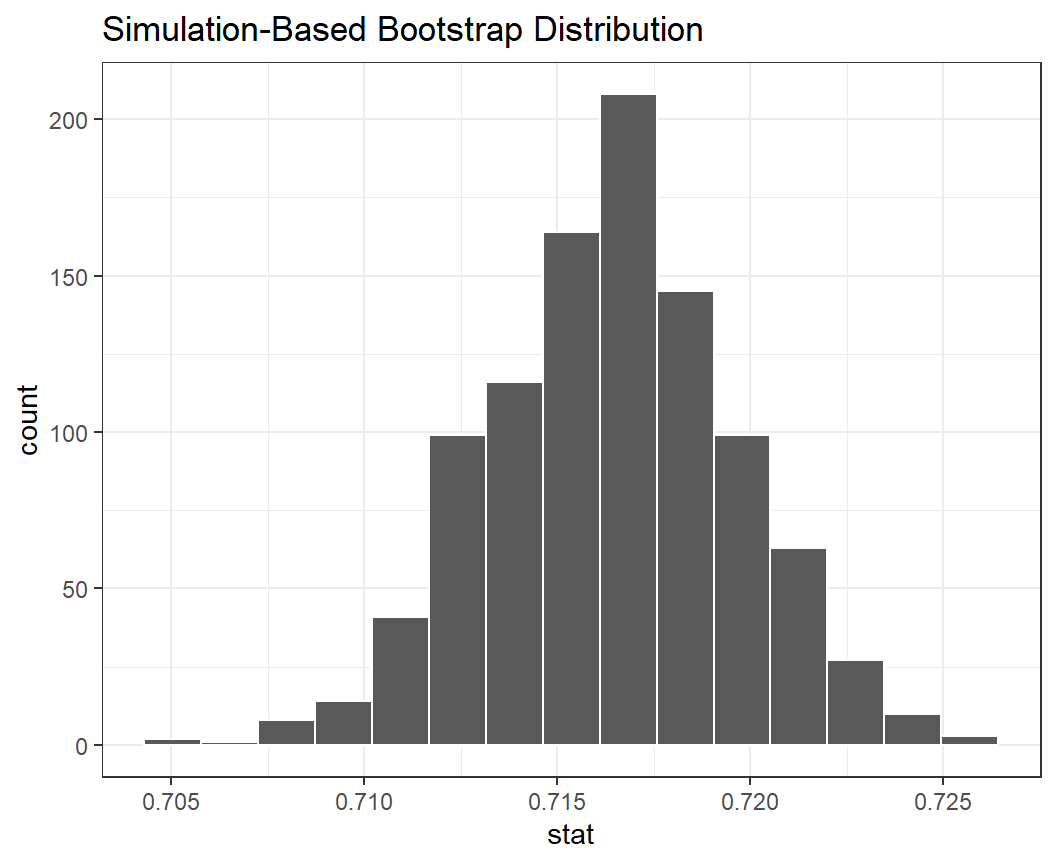
ic_perc_licencia_curso <-
  remuestreo_licencia_curso |>
  get_confidence_interval(level = 0.95, type = "percentile")
ic_perc_licencia_cursoremuestreo_licencia_curso |>
visualize() +
shade_confidence_interval(endpoints = ic_perc_licencia_curso)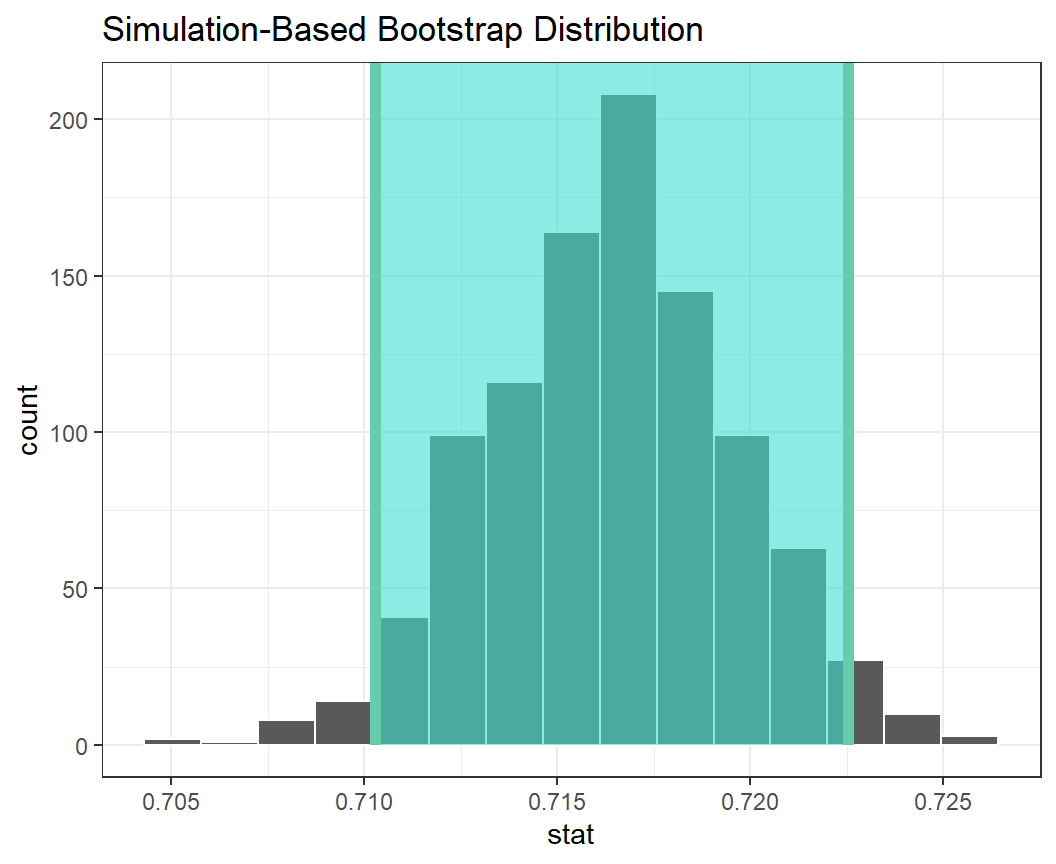
\[\hat{p}-Z_{\alpha/2}\sqrt{\frac{\hat{p}(1-\hat{p})}{n}} < p < \hat{p}+Z_{\alpha/2}\sqrt{\frac{\hat{p}(1-\hat{p})}{n}}\]
datos2 |>
count(licencia_curso)total_muestra <- datos2 |> nrow()
total_licencia_curso <- 13809
prop.test(
x = total_licencia_curso,
n = total_muestra,
conf.level = 0.95,
p = 0.5
)
    1-sample proportions test with continuity correction

data:  total_licencia_curso out of total_muestra, null probability 0.5
X-squared = 3611.4, df = 1, p-value < 2.2e-16
alternative hypothesis: true p is not equal to 0.5
95 percent confidence interval:
 0.7100256 0.7228026
sample estimates:
        p
0.7164574